ABC analysis in inventory management is the simple but powerful idea that not every SKU deserves the same attention. If you manage inventory in India, you already know the uncomfortable truth firsthand. The 200 items sitting quietly in your warehouse do not all tie up the same capital, move at the same speed, or hurt you equally when they go out of stock. Yet most growing businesses still apply a single, flat policy to their entire catalogue, counting everything with the same frequency, holding similar safety stock across the board, and chasing every shortage with equal urgency.
ABC analysis fixes the first half of that problem. ABC-XYZ analysis fixes the rest. Together, they give you a structured way to decide where to spend your control effort, your working capital, and your team’s time, which matters far more in a market where capital is expensive, demand swings with festive cycles, and a single dead-stock SKU can quietly eat your margins for a year.
This guide walks through both methods from first principles, with worked examples in rupees, an India-specific lens, and a downloadable Excel template you can drop your own data into today.
What Is ABC Analysis in Inventory Management?
ABC analysis in inventory management is a method of classifying inventory into three categories based on the value each item contributes to your business, most commonly its annual consumption value (unit cost multiplied by annual demand). The logic rests on the Pareto principle, the familiar 80/20 rule: a small fraction of your SKUs typically accounts for the overwhelming majority of your inventory value.
The full form of ABC analysis is Always Better Control — the technique was developed as a way to apply better, more selective control over inventory rather than treating every item the same. So the simple meaning of ABC analysis is this: rank items by importance, then control each class differently. It is also called the ABC classification method or the ABC technique of inventory control, and the same logic appears in cost accounting, materials management, and the pharmacy and pharmaceutical supply chain.
The ABC analysis formula for each item is straightforward:
Annual consumption value = Unit cost × Annual demand (units)
You then rank every SKU by that value, calculate each item’s cumulative percentage of total inventory value, and cut the list into three classes.
The three classes work like this:
Class A items are your vital few in ABC analysis, A represents the high-value items that justify the tightest control. They usually represent around 70–80% of total annual consumption value while making up only 10–20% of your SKU count. These are the items you watch closely, count often, and never want to run out of.
Class B items are the middle tier. They account for roughly 15–25% of value and a similar share of SKUs. They deserve moderate, periodic attention.
Class C items are the trivial many. They make up the bulk of your catalogue, often 50% or more of SKUs, but the percentage of total inventory value held by C-category material is usually only about 5%. The goal here is to spend as little management effort as possible while keeping availability acceptable.
The percentages are conventions, not laws. Your actual breakpoints will depend on your business; the method is about the ranking and the cut, not memorising 80/15/5.
Why ABC Analysis in Inventory Management Matters for Indian Businesses
The theory is universal, but a few realities make ABC analysis in inventory management especially valuable in the Indian context.
Working capital is expensive here. With borrowing costs and the pressure on cash flow that most SMEs and D2C brands feel, the capital locked in slow C-class stock is rarely free money. Knowing precisely which 15% of items hold most of your value lets you negotiate harder on those, hold them tighter, and stop over-ordering the long tail.
Demand is seasonal and spiky. Festive surges around Diwali, wedding seasons, end-of-financial-year buying, and quick-commerce demand spikes mean an item that is sleepy for ten months can dominate for two. ABC alone does not capture this, which is exactly why ABC-XYZ, covered below, matters so much in India.
SKU counts are exploding. As brands list across multiple marketplaces, Amazon, Flipkart, Meesho, Myntra, Nykaa, ONDC, and their own D2C storefronts, catalogues balloon and the long tail grows faster than anyone can manage by hand. Classification is the only sane way to keep control. (If you are juggling stock across channels, our guide to multi-warehouse inventory management pairs naturally with this one.)
How to Perform ABC Analysis in Inventory Management: Step by Step
You can run a basic ABC analysis in inventory management in a spreadsheet in under an hour. Here is the process the template automates for you.
Step 1: List every SKU with its unit cost and annual demand. Pull twelve months of consumption or sales data. Annual demand is the number of units consumed or sold over the year.
Step 2: Calculate annual consumption value. For each item, multiply unit cost by annual demand. A part costing ₹250 that you consume 4,000 units of has an annual value of ₹10,00,000.
Step 3: Sort items from highest value to lowest. This single sort is where the Pareto pattern reveals itself.
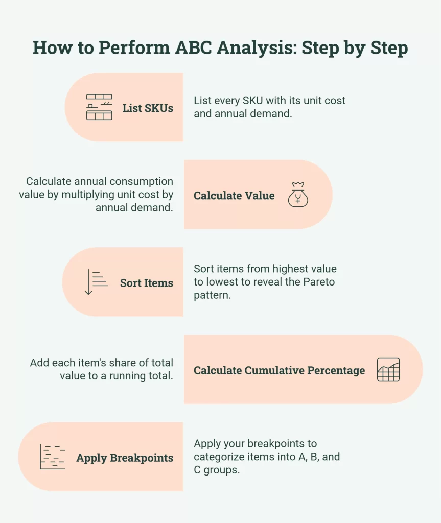
Step 4: Calculate the cumulative percentage of value. Running down the sorted list, add each item’s share of total value to a running total.
Step 5: Apply your breakpoints. Items accumulating up to ~80% of value are Class A; the next ~15% are Class B; the final ~5% are Class C. Adjust the cut points to fit how your value actually distributes.
Imagine a mid-sized electronics distributor with ten representative SKUs:
| SKU | Unit Cost (₹) | Annual Demand | Annual Value (₹) |
|---|---|---|---|
| Smartphone module | 8,500 | 1,200 | 1,02,00,000 |
| Display panel | 4,200 | 1,500 | 63,00,000 |
| Battery pack | 1,100 | 3,000 | 33,00,000 |
| Circuit board | 2,300 | 900 | 20,70,000 |
| Charger unit | 450 | 6,000 | 27,00,000 |
| Cable assembly | 90 | 18,000 | 16,20,000 |
| Casing | 220 | 5,000 | 11,00,000 |
| Screw kit | 12 | 40,000 | 4,80,000 |
| Sticker set | 5 | 30,000 | 1,50,000 |
| Foam insert | 8 | 12,000 | 96,000 |
Sort by annual value and accumulate, and a clear pattern emerges. The smartphone module, display panel, battery pack, and charger unit, four of ten SKUs, together hold roughly 80% of the total value. These are your Class A items. The circuit board, cable assembly, and casing form the Class B middle. The screw kit, sticker set, and foam insert, high in unit count but tiny in value, are textbook Class C. You would never want to discover you are physically counting 40,000 screws as carefully as you count 1,200 smartphone modules. ABC analysis tells you not to.
Setting Inventory Control Policies by Class
ABC analysis in inventory control is only useful if it changes what you actually do. The whole point of the ABC technique of inventory control is to apply a different policy to each class. Here is how that should differ across the three.
For Class A, control is tight and frequent. Review stock levels often, keep safety stock lean but reliable, forecast demand carefully, and build close relationships with these suppliers. Cycle count these items most frequently, weekly or even daily for the very top items, because an error here is expensive. Our guide on cycle counting versus physical inventory explains how to schedule counts by class rather than shutting the warehouse for an annual blanket count.
For Class B, apply moderate, periodic control. Monthly review cycles, standard safety stock, and routine reordering usually suffice. Watch for items drifting toward A or C and reclassify them when they do.
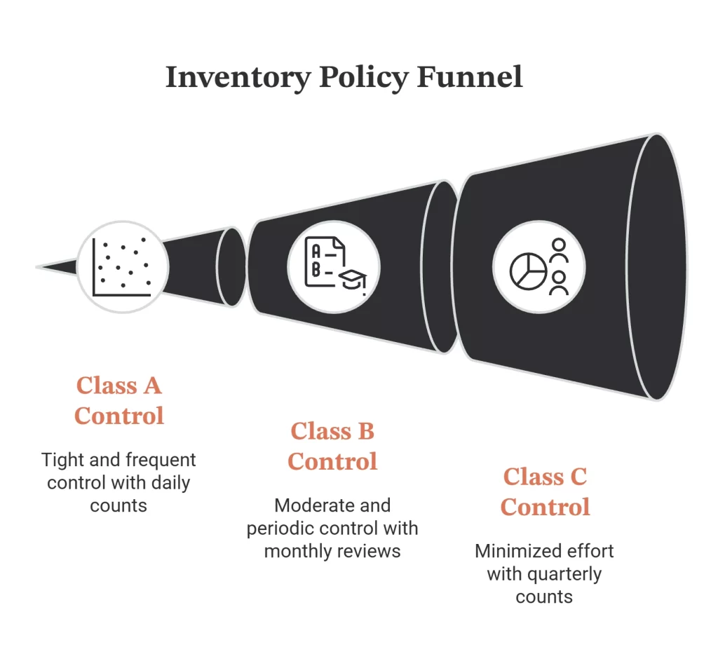
For Class C, minimise effort. Order in larger, less frequent batches to reduce ordering overhead, hold generous safety stock (it is cheap), and automate replenishment so nobody has to think about these items day to day. Counting quarterly is often enough.
This is also where reorder point discipline pays off: A items warrant carefully calculated reorder points, while C items can run on simple min-max rules.
Advantages and Disadvantages of ABC Analysis
Like any technique, ABC analysis has clear strengths and real limits, and knowing both keeps you from over-trusting it.
The advantages of ABC analysis are compelling. It focuses scarce attention and working capital where they matter most, improves inventory turnover by stopping over-investment in the long tail, sharpens cycle-counting and reorder-point decisions, and is simple enough to run in a spreadsheet yet powerful enough to scale across thousands of SKUs. For Indian businesses watching every rupee of working capital, that focus is the single biggest payoff.
The disadvantages of ABC analysis are just as important. It looks only at value and ignores demand variability, criticality, and lead time, so a cheap-but-critical part can be misclassified as unimportant. It is a static snapshot that goes stale as demand shifts, and it offers no guidance on how to forecast the erratic items it flags. These gaps are exactly why ABC is usually paired with a second dimension — most powerfully with XYZ analysis, covered below.
ABC vs VED vs SDE: Related Classification Methods
ABC is the best-known inventory classification method, but it is not the only one, and the others answer questions ABC cannot. VED analysis classifies items as Vital, Essential, or Desirable based on how critical they are to operations — widely used in pharmacy, hospital, and pharmaceutical inventory where a cheap missing item can stop everything. SDE analysis in inventory management classifies items as Scarce, Difficult, or Easy to procure, focusing on supply availability and lead time. Many mature operations run ABC for value, VED for criticality, and SDE for supply risk, then combine them. For most businesses, though, the highest-leverage pairing is ABC with XYZ.
The Limitation of ABC Alone
Here is the gap that catches most businesses out. ABC analysis ranks items purely by value. It says nothing about how predictable their demand is.
Consider two Class A items of equal annual value. One sells steadily, roughly the same volume every week, easy to forecast, low risk. The other is wildly erratic, flat for months, then a festive explosion, then flat again. ABC treats them identically. But they could not be more different to manage. The steady item can run on lean safety stock and tight reorder points. The erratic one will either stock out during its spike or drown you in dead stock if you over-prepare.
In India, where demand variability is the norm rather than the exception, ignoring this dimension is genuinely dangerous. That is the problem XYZ analysis solves.
What Is XYZ Analysis?
XYZ analysis classifies items by demand variability, how predictable or erratic their consumption is over time. It is the perfect complement to ABC’s value lens.
Class X items have stable, predictable demand. Consumption barely fluctuates from period to period, so forecasting is easy and accurate. These are the items you can manage with confidence and minimal buffer.
Class Y items have variable demand, often with identifiable patterns, seasonal trends, festive peaks, or gradual growth. Forecastable, but with meaningfully more uncertainty than X.
Class Z items have erratic, irregular demand with no reliable pattern. Sporadic orders, one-off spikes, long quiet stretches. Forecasting is hard and error-prone, so these carry the highest stocking risk.
The standard way to measure variability is the coefficient of variation (CV), the standard deviation of demand divided by the mean demand, across your time periods (usually the twelve months of the year). A low CV means stable demand; a high CV means erratic demand.
A common set of breakpoints is: CV below 0.5 is Class X, CV between 0.5 and 1.0 is Class Y, and CV above 1.0 is Class Z. As with ABC, treat these as starting points and tune them to your data.
Combining Them: The ABC-XYZ Matrix
When you overlay the two classifications, you get a nine-box matrix, every item lands in one of nine cells, from AX to CZ. This is where the real management insight lives, because each cell implies a distinct strategy.
| X (stable) | Y (variable) | Z (erratic) | |
|---|---|---|---|
| A (high value) | AX | AY | AZ |
| B (mid value) | BX | BY | BZ |
| C (low value) | CX | CY | CZ |
Reading the matrix:
AX: high value, predictable. Your dream items. High value but easy to forecast, so you can run them lean with tight reorder points and minimal safety stock. Automate replenishment and enjoy the reliability. Focus your forecasting precision here because the capital at stake is large.
AY: high value, variable. Important and somewhat unpredictable. Combine careful forecasting with sensible safety stock, and watch them closely, especially around known seasonal peaks. Most festive-sensitive hero products live here.
AZ: high value, erratic. The danger zone. Big money tied to unpredictable demand. These items deserve your most senior attention: make-to-order where possible, tight supplier coordination, and conservative but deliberate buffering. Do not automate these blindly.
BX and BY are your steady operational middle, standard policies, periodic review, mostly automatable.
BZ and CZ are erratic items where you accept the unpredictability. For CZ (low value, erratic), the cheapest answer is usually to hold a comfortable buffer and stop worrying, the stock is inexpensive and the management cost of precision exceeds the benefit.
CX: low value, predictable. Perfect candidates for full automation and bulk ordering. Set a simple rule and forget them.
For a fashion or seasonal business, this matrix is transformative. A hero kurta line might be AY: high value, festival-driven. Basic packaging is CX. A niche limited-edition piece is AZ or CZ. Our piece on seasonal inventory management for fashion brands goes deeper on managing those festive swings, and demand-driven replenishment explains how to react to actual pull rather than stale forecasts.
Worked ABC-XYZ Example
Return to the electronics distributor. The battery pack and charger unit are both healthy Class A or B items by value. But suppose the battery pack sells at a steady ~250 units a month (low CV, Class X) while the charger unit spikes hard every festive quarter and goes quiet otherwise (high CV, Class Z).
The battery pack is BX, manage it with lean buffers and automated reordering. The charger unit is BZ, same value tier, completely different handling. You will want to pre-position stock ahead of its known spikes, coordinate with the supplier on lead times, and accept a larger seasonal buffer that you deliberately draw down rather than carry year-round. ABC alone would have told you to treat these two identically. ABC-XYZ tells you the truth: same wallet impact, opposite playbook.
Common Mistakes to Avoid
A few traps catch businesses repeatedly. Treating the classification as permanent is the biggest one, demand shifts, products mature, and an A item this year may be a C next year. Re-run the analysis quarterly, or at minimum every six months.
Using only one criterion when several matter is another. Annual value is the standard ABC input, but for some businesses criticality (a cheap part that halts production if missing), lead time, or margin matters more than raw consumption value. You can run ABC on whichever criterion drives your risk, or run it on several and combine.
Ignoring the demand dimension entirely, running ABC and stopping there, leaves the seasonal risk that is so acute in India completely unmanaged. And finally, classifying but not changing your policies wastes the whole exercise. The output is not the chart; it is a different way of ordering, counting, and buffering each class.
These mistakes sit alongside the broader patterns we cover in costly inventory management mistakes, worth a read once you have your classes set.
From Spreadsheet to System
A spreadsheet is the right place to learn ABC-XYZ and to run it the first few times. But once your catalogue crosses a few hundred SKUs across multiple channels and warehouses, manual reclassification every quarter becomes its own full-time job, and the data goes stale between runs.
This is where a warehouse management system earns its keep. A capable WMS can classify continuously against live transaction data, drive cycle-count frequency automatically by class, flag items drifting between categories, and apply class-specific replenishment rules without anyone re-sorting a spreadsheet. The analysis stops being a periodic project and becomes a living layer over your operations. Connecting it to your reorder point and replenishment logic closes the loop entirely.
Start with the template below. Once the method is paying off and the manual upkeep starts to bite, that is your signal to move it into a system.
How to Use the Free Excel Template
The accompanying workbook does all the maths described above. Drop your SKU list, unit costs, and twelve months of demand into the input sheet, and it automatically calculates annual value, ABC class, the coefficient of variation, XYZ class, and the combined ABC-XYZ cell for every item, colour-coded so the pattern jumps out. Sample data is pre-loaded so you can see exactly how it behaves before replacing it with your own numbers. The breakpoints are editable in one place, so you can tune the cut-offs to your business in seconds.
Conclusion
ABC analysis tells you where your money is. XYZ analysis tells you where your risk is. Used together, they replace one-size-fits-all inventory management with a focused strategy that puts your scarce attention, capital, and counting effort exactly where they earn the most return, which, in a high-cost-of-capital, deeply seasonal market like India, is not a nice-to-have but a competitive edge. Download the free Excel template below, run ABC analysis in inventory management on your own catalogue, and re-run it every quarter to keep your control where it belongs.
Frequently Asked Questions
Quarterly is a good default for most Indian businesses, and essential if you are seasonal. At minimum, re-run every six months. Demand patterns and product lifecycles shift faster than people expect, and a stale classification quietly misallocates your control effort.
That is precisely what the matrix captures. A high-value, low-volume item with erratic demand lands in AZ: flagged for your closest attention and conservative, deliberate buffering rather than blind automation.
Yes. Value is the standard, but you can classify on margin, criticality, lead time, or any factor that drives your risk. Many businesses run ABC on value and again on criticality, then combine the two views.
Even more so. With limited working capital and a lean team, knowing exactly where to focus is the difference between healthy cash flow and money trapped in dead stock. The spreadsheet costs you an hour. Our guide to WMS for small businesses in India covers the next step once you outgrow manual analysis.
ABC analysis is a practical application of the Pareto principle. Pareto describes the 80/20 distribution; ABC turns that observation into three actionable classes with distinct management policies. ABC analysis is most closely associated with Pareto, which is why it is sometimes called Pareto-based inventory classification.
The full form of ABC analysis is Always Better Control. Its meaning is simple: classify inventory into A, B, and C groups by value, then apply progressively lighter control as you move from A to C. In short, A items are tightly controlled, B items moderately, and C items loosely.
In ABC analysis, A represents the highest-value items typically the top 70–80% of annual consumption value held in just 10–20% of SKUs. A items are the few products that tie up most of your money, so they get the closest forecasting, tightest reorder points, and most frequent cycle counts.
Yes. The same ABC classification logic is used in cost accounting and materials management to prioritise items by value for control, valuation, and review, not just in the warehouse.

Kapil Pathak is a Senior Digital Marketing Executive with over four years of experience specializing in the logistics and supply chain industry. His expertise spans digital strategy, search engine optimization (SEO), search engine marketing (SEM), and multi-channel campaign management. He has a proven track record of developing initiatives that increase brand visibility, generate qualified leads, and drive growth for D2C & B2B technology companies.